GIS Infrastructure for Management (JHU AAP SPRING 2025)

cartography, Graphics

Midterm project: “All K-12 Schools, both public and private. Suggest other locations for K-12 schools near the JHU Homewood campus.”

To view the full paper, click the hyperlinked title:

Final Project: “Develop a GIS vision for a local government, company or higher education institution, that doesn’t currently have one, anywhere in the State of Maryland.  Research the required components to put it into place and create a proposed starting budget, governance document and assigned staff.   Create a spatial overlay to perform initial analysis of the chosen location.”

To view the full paper, click the hyperlinked title below:

Cartogram

cartography, Graphics

The purpose of this assignment is “to produce a color, noncontiguous
cartogram of the Hispanic or Latino Population in the United States based on the [latest] US Census data.”

Lab9_RaoelisonFitia

Compare the Hispanic Population Cartogram to the Standard U.S. Map:

  • Which state has the largest Hispanic population and which state has the smallest population?  How can you tell?
    • The state that has the largest Hispanic Population is California and the state that has the smallest Hispanic Population is Vermont. Based on the exploding size compared to Texas and Florida (which are also big), California has the largest population compared to the rest of the country. Vermont has over 600,000 total persons but the Hispanic population (less than 10,000) is small compared to the total.
  • Find Maryland on the cartogram.  Does it appear smaller or larger relative to its size on the standard map?
    • It’s larger because it has over 470,000 Hispanic persons/10,000 sq. mi (which means 1 in 47 in 100 miles squared) compared to other states like Vermont, Wyoming, etc.
  • Based on the cartogram you created, which three states would you conclude have the most Hispanic representatives?
    • California, Texas, and Florida
  • In conclusion, do you think the cartogram effectively convey the underlying message, in this case Hispanic population, to the audience?  Explain.
    • Yes. The enlargement/shrinking size and color shading of the symbols is direct to the point and tells the map reader right away the information they need to know.

Data Classification & Chloropleth Mapping

cartography, Graphics

The objective of this project is to “investigate various options for classifying quantitative data and create four different choropleth maps of population data by county . . . using the 2014 population data [obtained] from the U.S. Census Bureau.”

Lab6_RaoelisonFitia

Challenges/Disadvantages: 

  • Map title – Since all maps display population density, I could’ve used different classification methods, map title could be, “The effects of Data Classification on Choropleth Maps” and add a subtitle: “2017 Wisconsin Population Density by County” to the layout.
  • Legend seems to contradict with the values.
  • Maps are distorted thus unclear projection.
  • Did not use standardized data for choropleth mapping (i.e., Population density rather than total population). Instead, I used raw data for choropleth mapping.
  • The word “Legend” was not removed and the area unit for density was not specified.
  • Increase the legend & font size. Specify the area unit for density.
  • If I scaled the maps properly, I would  have more space available on the layout.
  • Did not include a brief description of each classification method to emphasize map purpose and to help the audience understand how to interpret the map.

Comparing these four classification methods, I see a difference between the divide in attribute values and the value range. For example, with Quantile, the values are linear, the features are grouped in equal numbers and the distortion of the map can determine how many class values can you use. It is similar to Equal Interval however, it divides the range of attribute values into equal-sized subranges, which allows the user to specify the number of intervals, and ArcGIS can automatically determine the class breaks based on the value range (e.g 0–100, 101–200, and 201–300). If I had not used standardized data, it would’ve been easier for me to determine which classification best represent the data of map well. If it were only raw data, I would say Natural Breaks  because the classes were divided in a way whose boundaries are set where there are relatively big differences in the data values. This project was hard for me to understand at first because I wasn’t sure I should have modified the values for each classification method, hence why each map looks distorted and doesn’t seem to match the data.

Map Projections

cartography, Graphics

The objective of this lab was to “improve [our] conceptual understanding of Map Projections . . . using Geographic Information System to transform the world from one map projection into another.”

Lab3_RaoelisonFitia

For the first map application (North America Equidistant Conic) – One of the requirements for this map application was to choose a projection to look like “a little globe” and “show the route”. The (Sphere) Robinson Projection is a compromise projection, hence it does not preserve any properties. The best projection for this map application would be an azimuthal equidistant projection because both distance and direction are accurate from the central point. What I could’ve done differently is not moving the central meridian to 74W (Bogota) or 76o W (Baltimore) to maintain an accuracy (distance measurement) between these two cities, and adjust the latitude of origin (point of tangency) to the location of Bogota (5N) or Baltimore (39N).

For the second map application (South Pole Azimuthal Equidistant) – the projection property was missing, and although my justification was correct, it is not clearly reflected by the Tossot Ellipses shown on the map.

For the third map application (Sphere Mollweide) – this needed an equal area projection despite that Mollweide is an equal-area projection, it distorted the shape of the U.S. What could’ve been done differently is adjusting the central meridian.

For the fourth map application (Cylindrical Equal Area World) – The purpose is to ‘generate a world map projection that does not distort areas.’ however, the map should’ve shown the whole world, not just the U.S. It was also missing the projection property. Another mistake is that the Cylindrical projection greatly distorts areas in the high latitudes.  To fix this, I could’ve tried other projections that also preserve shape & area, i.e., Pseudocylindrical equal-area projection -> Sinusoidal projection, homolosine projection, etc.

For the fifth map application (Sphere Wagner V) – It needed a compromise projection such as Sphere Robinson Projection, which does not preserve properties but gives an appealing look for the audience.

For the sixth map application (Sinusoidal World) – The purpose of this application was to show the weirdest projection but my justification didn’t really serve that purpose.

Overall, this lab was one of the challenging tasks I’ve had because while map projections are not my forte, I tried my best to fulfill the objective as best as I could and as much I know/learned about map projections.

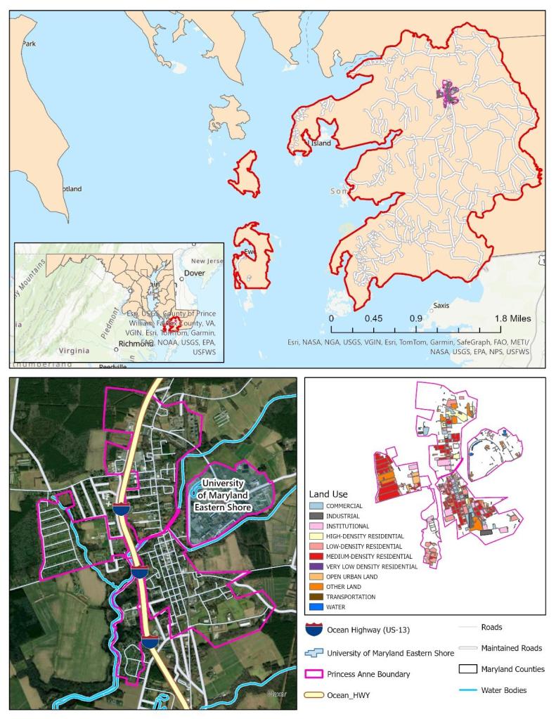
Map Composition

cartography, Graphics

I was given a file that contained map elements and data that needed to be arranged in Adobe Illustrator. My objective was to construct a well-balanced map on Illustrator by using the map elements and data I was given, and organize them neatly.

Lab01_RaoelisonFitia The first thing I decided to change in one of the elements was the color scheme of the map. Initially, the Texas map had different colors that I felt did not reflect well with the data on the legend so I chose a different color scheme that can reflect the numbers. However, my choice of color scheme became a drawback as the two dark colors look closely similar to each other that it is difficult to distinguish between the two. This design choice made it hard for the viewer to read and understand the map.

In this project, a neatline 7′ x 9′ was required to make this map. I felt that the neatline was helpful and beneficial as it compresses the space needed to be filled in a map. It helped me resize and arrange the elements faster.

One of my strengths in this map was resizing the inset maps and aligning properly to create a good and logical connection with the main map. Another strength was making use of the space and made sure I didn’t leave a big empty space that could mess with the balance of the map.

Despite the strengths that was shown well in this project, it also brought disadvantage to the readers. There were some qualities I didn’t consider while making this map which were adjusting the spacing between the colored boxes in the legend and making the scale bar proportional to the main map in order to bring balance. I also used up a lot of space which makes it hard for the reader to rest their eyes on the map.

Overall, this project was a good learning experience and taught me the importance of cartography in the geography field which is to create maps as effective communication tools for the audience to see, read, and understand.